R tutorial
From Organic Design wiki
Contents
Resources
- Quickest way to learn R: use the Contributed Documentation (http://cran.stat.auckland.ac.nz/other-docs.html)
- Thousands of pages of documentation including short guides / reference cards
- Contributed guides for the beginner
- A Guide for the Unwilling S User (http://cran.stat.auckland.ac.nz/doc/contrib/Burns-unwilling_S.pdf)
- R for Beginners (http://cran.stat.auckland.ac.nz/doc/contrib/Paradis-rdebuts_en.pdf)
- Reference card (http://cran.stat.auckland.ac.nz/doc/contrib/refcard.pdf)
- More comprehensive contributed guides
- Using R for Data Analysis and Graphics (http://cran.stat.auckland.ac.nz/doc/contrib/usingR-2.pdf)
- Simple R (http://cran.stat.auckland.ac.nz/doc/contrib/Verzani-SimpleR.pdf)
- S programming techniques (http://www.stat.auckland.ac.nz/S-Workshop/Ihaka/lecture.pdf)
Obtaining help in R
help.start()           # Browser based help documentation
help()                 # Help on a topic (note: help pages have a set format)
? ls                   # alternative help method on ls function
apropos(mean)          # Find Objects by (Partial) Name
example(mean)          # Run an Examples Section from the Online Help
demo()                 # Demonstrations of R Functionality
demo(graphics)         # Demonstration or graphics Functionality
RSiteSearch()          # Searches web newslist archives and retrieves results using http
- There objects are functions, to run them you must put parentheses '()' after the function name
Useful commands in the R environment
search()              # Give Search Path for R Objects
searchpaths()         # Give Full Search Path for R Objects
ls()                  # List objects
objects()             # alternate function to list objects
data()                # Publically available datasets
rm()                  # Remove Objects from a Specified Environment
save.image()          # Save R Objects
q()                   # Terminate an R Session →  prompted to Save workspace image? [y/n/c]:
Command prompt
- Type commands after the prompt (>) e.g.
> x <- 1:10        # assignment of 1 to 10 to an object called 'x'
> x                # Returning the x object to the screen
 [1]  1  2  3  4  5  6  7  8  9 10
- Continuation of commands is expected after the plus symbol (+) e.g.
> x <- 1:          # partial command → parser is expecting more information
+  10
> x
 [1]  1  2  3  4  5  6  7  8  9 10
- Text following a '#' is commented out
Basic (atomic) data types
- Logical
T                 # TRUE
F                 # FALSE
- Numeric
3.141592654 # Any number [0-9\.]
- Character
"Putative ATPase" # Any character [A-Za-z] must be single or double quoted
- Missing values
NA # Label for missing information in datasets
- See also help("NA"), help("NaN")
Assignment of objects
- objects must start with a letter [A-Z a-z]
- "<-" The arrow assigns information to the object on the left
x <- 42                # Assignment to the left
x
x = 42                 # Equivalent assignment (not recommended)
x
42 -> x                # Assignment to the right
x
Saving objects
getwd()                        # Returns the current directory where R is running
setwd("C:/DATA/Microarray")    # Set the working directory to another location
getwd()                        # Check the directory has changed
x <- 42
save.image()                   # Saves a snapshot of objects to file .RData
y <- x * 2                     # Make a new object called 'y'
y                              # Return value of 'y'
q()                            # quit R
Restart R by double clicking on the file .RData in C:/DATA/Microarray
x              # Returns 'x' as it was saved to .RData in "C:/DATA/Microarray"
y              # 'y' should not exist
Object data types
- Create a scalar (vector of length 1)
a <- 3.14            # Assign pythagorus to object 'a'
length(a)            # The scalar is actually a vector of length 1
pi                   # Already have a built in object for pythagorus
search()             # Print the search path for all objects
find("pi")           # "pi" is located in package:base
- Create a vector
x <- c(2,3,5,2,7,1)  # Numbers put into a vector using 'c' function concatenate
x
y <- c(10,15,12)
y
names(y) <- c("first","second","third")    # Elements can be given names
z <- c(y,x)
z
- Create a matrix
zmat <- cbind(x,y)   # cbind joins vectors together by column
zmat
- Whats going on in the second column → number recycling
mat <- matrix(1:20, nrow=5, ncol=4)                   # Constructing a matrix
mat
colnames(mat) <- c("Col1","Col2", "Col3", "Col4")     # Adding column names
mat
- Create a list
mylist <- list(1:4,c("a","b","c"), LETTERS[1:10])
mylist
mylist <- list("element 1" = 1:4,"second vector" = c("a","b","c"), "Capitals" = LETTERS[1:10])
mylist
Indexing
- Subsetting a vector
x[c(1,2,3)]                     # Selecting the first three elements of 'x'
x[1:3]                          # Same subset using ':' sequence generation → see help(":")
y[2]                            # Selecting the second element of 'y'
y["second"]                     # Selecting the second element of 'y' (by name)
- Subsetting a matrix
mat[,1:2]                       # Selecting the first two columns of 'mat'
mat[1:2, 2:4]                   # Selecting a subset matrix of 'mat'
- Subsetting a list
mylist[[1]]                    # Subsetting list 'mylist' by index
mylist[["element 1"]]          # Subsetting list 'mylist' by name 'element 1'
mylist$"element 1"             # Alternate way of subsetting
mylist$Capitals[1:5]           # Selecting the first five elements of 'Capitals' in 'mylist' (case sensitive)
Plotting data
- See help pages for basic plot functions
help(plot)
help(par)
example(plot)
par(ask=TRUE)         # Set the printing device to prompt user before displaying next graph
example(hist)
Reading / writing files
- Reading data
help(scan)
help(read.table)
- Reading a GPR file header using scan
dataDir <- "C:/DATA/Microarray/GPR")
mydata <-  scan(file.path(dataDir, "BE34.gpr"), what="", nlines=29)  # Get first 29 rows of data
mydata
- Reading a GPR file data section using read.table
colClasses <- rep("NULL", 82)
colClasses[c(1:5, 9,12, 18, 21)] <- NA                                      # Set colClasses to ignore unwanted columns
mydata <- read.table(file.path(dataDir,"BE34.gpr"), header=T,  sep="\t",
                                  nrows=20, skip=31, colClasses=colClasses) # Get first 20 lines of data after 31st row
mydata
- Writing data
help(write)
help(write.table)
- See also dump, restore, save, load
User defined functions
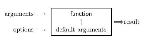
- Writing functions provide a means of adding new functionality to the language. A function has the form:
myfun <- function( arglist ){ body }

- Identity function: returns its input arguement
myfun <- function(x){x}        # Creating identity function
myfun("foo")                   # Running the function
myfun()                        # Fails: no input arguement provided
- A simple function
square <- function(x){x * x}         # Square the input number
square(10)                  # Returns 10 squared
square(1:4)              # Underlying arithmetic is vectorized
- Graphical example from user defined function
- The following function generates data from sine distributions and examines
bias variance tradeoff of a smoothing function using different smoothing parameters. Paste it into R
"biasVar" <- function(df1=4,  df2=15,  N = 100,  seed=1)
{
 set.seed(seed)
 # 1) Data setup
 ylim <- c(-2,2)
 xlim <- c(-3,3)
 par(mfrow=c(2,2), mar=c(5,4,4-2,2)+0.1,mgp=c(2,.5,0) )
 x <- rnorm(80, 0, 1)
 y <- sin(x) + rnorm(80, 0, 1/9)
 xno   <- 500
 sim <- matrix(NA, nc=N, nr=xno)
 xseq <- seq(min(x),max(x), length=xno)
 plot(x, y, main=paste("df=",df1,sep=""), xlim=xlim, ylim=ylim)    # Using Splines
 truex <- seq(min(x), max(x), length = 80)
 lines(truex, sin(truex), lty = 5)
 splineobj <- smooth.spline(x, y, df = df1)
 lines(splineobj, lty = 1)
 plot(x, y, main=paste("df=",df2,sep=""), xlim=xlim, ylim=ylim)    # Using Splines
 truex <- seq(min(x), max(x), length = 80)
 lines(truex, sin(truex), lty = 5)
 splineobj <- smooth.spline(x, y, df = df2)
 lines(splineobj, lty = 1)
 plot(x, y, main=paste("Bias-Variance tradeoff, df=",df1, sep=""), type="n", xlim=xlim, ylim=ylim)
 for(i in seq(N))
   {
     x <- rnorm(80, 0, 1)
     y <- sin(x) + rnorm(80, 0, 1/9)
     splineobj <- smooth.spline(x, y, df = df1)
     sim[,i] <- predict(splineobj,xseq)$y
   }
 ci <- qt(0.975, N) * sqrt(apply(sim,1, var))
 bias <- apply(sim,1, mean)
 rect(xseq,bias-ci,xseq,bias+ci, border="grey")
 rect(xseq,sin(xseq),xseq,bias, border="black")
 lines(truex, sin(truex))
 plot(x, y, main=paste("Bias-Variance tradeoff, df=",df2,sep=""), type="n", xlim=xlim, ylim=ylim)
 for(i in seq(N))
   {
     x <- rnorm(80, 0, 1)
     y <- sin(x) + rnorm(80, 0, 1/9)
     splineobj <- smooth.spline(x, y, df = df2)
     sim[,i] <- predict(splineobj,xseq)$y
   }
 ci <- qt(0.975,N) * sqrt(apply(sim,1, var))
 bias <- apply(sim,1, mean)
 rect(xseq,bias-ci,xseq,bias+ci, border="grey")
 rect(xseq,sin(xseq),xseq,bias, border="black")
 lines(truex, sin(truex))
}
- Running the function
biasVar()                # Generates data from a sine curve looking at bias variance tradeoff
biasVar(df1=2, df2=30)   # Let's change the smoothing parameters in the function arguements
Quiting R
rm(list=ls())         # Cleaning up: Remove Objects from a Specified Environment
q()